How GPT Models Work

 

Introduction

It was 2021 when I wrote my first few lines of code using a GPT model, and that was the moment I realized that text generation had reached an inflection point. Prior to that, I had written language models from scratch in grad school, and I had experience working with other text generation systems, so I knew just how difficult it was to get them to produce useful results. I was fortunate to get early access to GPT-3 as part of my work on the announcement of its release within the Azure OpenAI Service, and I tried it out in preparation for its launch. I asked GPT-3 to summarize a long document and experimented with few-shot prompts. I could see that the results were far more advanced than those of prior models, making me excited about the technology and eager to learn how it’s implemented. And now that the follow-on GPT-3.5, ChatGPT, and GPT-4 models are rapidly gaining wide adoption, more people in the field are also curious about how they work. While the details of their inner workings are proprietary and complex, all the GPT models share some fundamental ideas that aren’t too hard to understand. My goal for this post is to explain the core concepts of language models in general and GPT models in particular, with the explanations geared toward data scientists and machine learning engineers.

How generative language models work

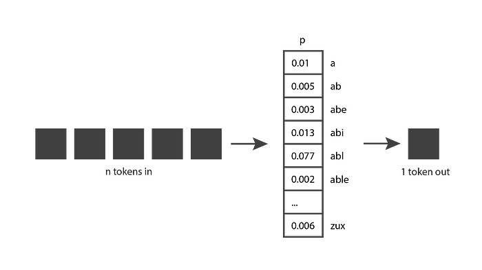
Let’s start by exploring how generative language models work. The very basic idea is the following: they take n tokens as input, and produce one token as output.

This seems like a fairly straightforward concept, but in order to really understand it, we need to know what a token is.

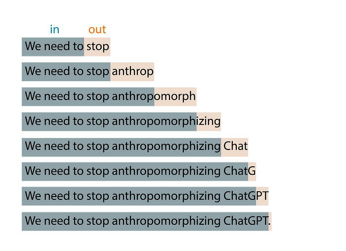
A token is a chunk of text. In the context of OpenAI GPT models, common and short words typically correspond to a single token, such as the word “We” in the image below. Long and less commonly used words are generally broken up into several tokens. For example the word “anthropomorphizing” in the image below is broken up into three tokens. Abbreviations like “ChatGPT” may be represented with a single token or broken up into multiple, depending on how common it is for the letters to appear together. You can go to OpenAI’s Tokenizer page, enter your text, and see how it gets split up into tokens. You can choose between “GPT-3” tokenization, which is used for text, and “Codex” tokenization, which is used for code. We’ll keep the default “GPT-3” setting.

You can also use OpenAI’s open-source tiktoken library to tokenize using Python code. OpenAI offers a few different tokenizers that each have a slightly different behavior. In the code below we use the tokenizer for “davinci,” which is a GPT-3 model, to match the behavior you saw using the UI.

import tiktoken

# Get the encoding for the davinci GPT3 model, which is the "r50k_base" encoding.
encoding = tiktoken.encoding_for_model("davinci")

text = "We need to stop anthropomorphizing ChatGPT."
print(f"text: {text}")

token_integers = encoding.encode(text)
print(f"total number of tokens: {encoding.n_vocab}")

print(f"token integers: {token_integers}")
token_strings = [encoding.decode_single_token_bytes(token) for token in token_integers]
print(f"token strings: {token_strings}")
print(f"number of tokens in text: {len(token_integers)}")

encoded_decoded_text = encoding.decode(token_integers)
print(f"encoded-decoded text: {encoded_decoded_text}")

text: We need to stop anthropomorphizing ChatGPT.
total number of tokens: 50257
token integers: [1135, 761, 284, 2245, 17911, 25831, 2890, 24101, 38, 11571, 13]
token strings: [b'We', b' need', b' to', b' stop', b' anthrop', b'omorph', b'izing', b' Chat', b'G', b'PT', b'.']
number of tokens in text: 11
encoded-decoded text: We need to stop anthropomorphizing ChatGPT.

You can see in the output of the code that this tokenizer contains 50,257 different tokens, and that each token is internally mapped into an integer index. Given a string, we can split it into integer tokens, and we can convert those integers into the sequence of characters they correspond to. Encoding and decoding a string should always give us the original string back.

This gives you a good intuition for how OpenAI’s tokenizer works, but you may be wondering why they chose those token lengths. Let’s consider some other options for tokenization. Suppose we try the simplest possible implementation, where each letter is a token. That makes it easy to break up the text into tokens, and keeps the total number of different tokens small. However, we can’t encode nearly as much information as in OpenAI’s approach. If we used letter-based tokens in the example above, 11 tokens could only encode “We need to”, while 11 of OpenAI’s tokens can encode the entire sentence. It turns out that the current language models have a limit on the maximum number of tokens that they can receive. Therefore, we want to pack as much information as possible in each token.

Now let’s consider the scenario where each word is a token. Compared to OpenAI’s approach, we would only need seven tokens to represent the same sentence, which seems more efficient. And splitting by word is also straighforward to implement. However, language models need to have a complete list of tokens that they might encounter, and that’s not feasible for whole words — not only because there are so many words in the dictionary, but also because it would be difficult to keep up with domain-specific terminology and any new words that are invented.

So it’s not surprising that OpenAI settled for a solution somewhere in between those two extremes. Other companies have released tokenizers that follow a similar approach, for example Sentence Piece by Google.

Now that we have a better understanding of tokens, let’s go back to our original diagram and see if we can understand it a bit better. Generative models take n tokens in, which could be a few words, a few paragraphs, or a few pages. And they produce a single token out, which could be a short word or a part of a word.

That makes a bit more sense now.

But if you’ve played with OpenAI’s ChatGPT, you know that it produces many tokens, not just a single token. That’s because this basic idea is applied in an expanding-window pattern. You give it n tokens in, it produces one token out, then it incorporates that output token as part of the input of the next iteration, produces a new token out, and so on. This pattern keeps repeating until a stopping condition is reached, indicating that it finished generating all the text you need.

For example, if I type “We need to” as input to my model, the algorithm may produce the results shown below:

While playing with ChatGPT, you may also have noticed that the model is not deterministic: if you ask it the exact same question twice, you’ll likely get two different answers. That’s because the model doesn’t actually produce a single predicted token; instead it returns a probability distribution over all the possible tokens. In other words, it returns a vector in which each entry expresses the probability of a particular token being chosen. The model then samples from that distribution to generate the output token.

How does the model come up with that probability distribution? That’s what the training phase is for. During training, the model is exposed to a lot of text, and its weights are tuned to predict good probability distributions, given a sequence of input tokens. GPT models are trained with a large portion of the internet, so their predictions reflect a mix of the information they’ve seen.

You now have a very good understanding of the idea behind generative models. Notice that I’ve only explained the idea though, I haven’t yet given you an algorithm. It turns out that this idea has been around for many decades, and it has been implemented using several different algorithms over the years. Next we’ll look at some of those algorithms.

A brief history of generative language models

Hidden Markov Models (HMMs) became popular in the 1970s. Their internal representation encodes the grammatical structure of sentences (nouns, verbs, and so on), and they use that knowledge when predicting new words. However, because they are Markov processes, they only take into consideration the most recent token when generating a new token. So, they implement a very simple version of the “n tokens in, one token out” idea, where n = 1. As a result, they don’t generate very sophisticated output. Let’s consider the following example:

If we input “The quick brown fox jumps over the” to a language model, we would expect it to return “lazy.” However, an HMM will only see the last token, “the,” and with such little information it’s unlikely that it will give us the prediction we expect. As people experimented with HMMs, it became clear that language models need to support more than one input token in order to generate good outputs.

N-grams became popular in the 1990s because they fixed the main limitation with HMMs by taking more than one token as input. An n-gram model would probably do pretty well at predicting the word “lazy” for the previous example.

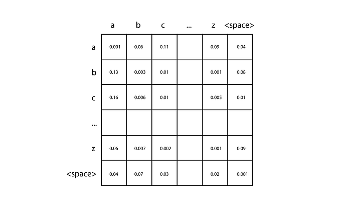
The simplest implementation of an n-gram is a bi-gram with character-based tokens, which given a single character, is able to predict the next character in the sequence. You can create one of these in just a few lines of code, and I encourage you to give it a try. First, count the number of different characters in your training text (let’s call it n), and create an n x n 2D matrix initialized with zeros. Each pair of input characters can be used to locate a particular entry in this matrix, by choosing the row corresponding to the first character, and the column corresponding to the second character. As you parse your training data, for every pair of characters, you simply add one to the corresponding matrix cell. For example, if your training data contains the word “car,” you would add one to the cell in the “c” row and “a” column, and then add one to the cell in the “a” row and “r” column. Once you have accumulated the counts for all your training data, convert each row into a probability distribution by dividing each cell by the total across that row.

Then to make a prediction, you need to give it a single character to start, for example, “c”. You look up the probability distribution that corresponds to the “c” row, and sample that distribution to produce the next character. Then you take the character you produced, and repeat the process, until you reach a stopping condition. Higher-order n-grams follow the same basic idea, but they’re able to look at a longer sequence of input tokens by using n-dimensional tensors.

N-grams are simple to implement. However, because the size of the matrix grows exponentialy as the number of input tokens increases, they don’t scale well to a larger number of tokens. And with just a few input tokens, they’re not able to produce good results. A new technique was needed to continue making progress in this field.

In the 2000s, Recurrent Neural Networks (RNNs) became quite popular because they’re able to accept a much larger number of input tokens than previous techniques. In particular, LSTMs and GRUs, which are types of RNNs, became widely used and proved capable of generating fairly good results.

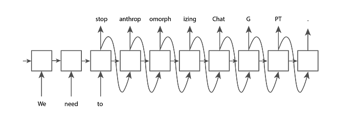
RNNs are a type of neural network, but unlike traditional feed-forward neural networks, their architecture can adapt to accepting any number of inputs and produce any number of outputs. For example, if we give an RNN the input tokens “We,” “need,” and “to,” and want it to generate a few more tokens until a full point is reached, the RNN might have the following structure:

Each of the nodes in the structure above has the same weights. You can think of it as a single node that connects to itself and executes repeatedly (hence the name “recurrent”), or you can think of it in the expanded form shown in the image above. One key capability added to LSTMs and GRUs over basic RNNs is the presence of an internal memory cell that gets passed from one node to the next. This enables later nodes to remember certain aspects of previous ones, which is essential to make good text predictions.

However, RNNs have instability issues with very long sequences of text. The gradients in the model tend to grow exponentially (called “exploding gradients”) or decrease to zero (called “vanishing gradients”), preventing the model from continuing to learn from training data. LSTMs and GRUs mitigate the vanishing gradients issue, but don’t prevent it completely. So, even though in theory their architecture allows for inputs of any length, in practice there are limitations to that length. Once again, the quality of the text generation was limited by the number of input tokens supported by the algorithm, and a new breakthrough was needed.

In 2017, the paper that introduced Transformers was released by Google, and we entered a new era in text generation. The architecture used in Transformers allows a huge increase in the number of input tokens, eliminates the gradient instability issues seen in RNNs, and is highly parallelizable, which means that it is able to take advantage of the power of GPUs. Transformers are widely used today, and they’re the technology chosen by OpenAI for their latest GPT text generation models.

Transformers are based on the “attention mechanism,” which allows the model to pay more attention to some inputs than others, regardless of where they show up in the input sequence. For example, let’s consider the following sentence:

In this scenario, when the model is predicting the verb “bought,” it needs to match the past tense of the verb “went.” In order to do that, it has to pay a lot of attention to the token “went.” In fact, it may pay more attention to the token “went” than to the token “and,” despite the fact that “went” appears much earlier in the input sequence.

This selective attention behavior in GPT models is enabled by a novel idea in the 2017 paper: the use of a “masked multi-head attention” layer. Let’s break down this term, and dive deeper into each of its sub-terms:

Attention: An “attention” layer contains a matrix of weights representing the strength of the relationship between all pairs of token positions in the input sentence. These weights are learned during training. If the weight that corresponds to a pair of positions is large, then the two tokens in those positions greatly influence each other. This is the mechanism that enables the Transfomer to pay more attention to some tokens than others, regardless of where they show up in the sentence.

Masked: The attention layer is “masked” if the matrix is restricted to the relationship between each token position and earlier positions in the input. This is what GPT models use for text generation, because an output token can only depend on the tokens that come before it.

Multi-head: The Transformer uses a masked “multi-head” attention layer because it contains several masked attention layers that operate in parallel.

The memory cell of LSTMs and GRUs also enables later tokens to remember some aspects of earlier tokens. However, if two related tokens are very far apart, the gradient issues could get in the way. Transformers don’t have that problem because each token has a direct connection to all other tokens that precede it.

Now that you understand the main ideas of the Transformer architecture used in GPT models, let’s take a look at the distinctions between the various GPT models that are currently available.

How different GPT models are implemented

At the time of writing, the three latest text generation models released by OpenAI are GPT-3.5, ChatGPT, and GPT-4, and they are all based on the Transformer architecture. In fact, “GPT” stands for “Generative Pre-trained Transformer.”

GPT-3.5 is a transformer trained as a completion-style model, which means that if we give it a few words as input, it’s capable of generating a few more words that are likely to follow them in the training data.

ChatGPT, on the other hand, is trained as a conversation-style model, which means that it performs best when we communicate with it as if we’re having a conversation. It’s based on the same transformer base model as GPT-3.5, but it’s fine-tuned with conversation data. Then it’s further fine-tuned using Reinforcement Learning with Human Feedback (RLHF), which is a technique that OpenAI introduced in their 2022 InstructGPT paper. In this technique, we give the model the same input twice, get back two different outputs, and ask a human ranker which output it prefers. That choice is then used to improve the model through fine-tuning. This technique brings alignment between the outputs of the model and human expectations, and it’s critical to the success of OpenAI’s latest models.

GPT-4 on the other hand, can be used both for completion and conversation, and has its own entirely new base model. This base model is also fine-tuned with RLHF for better alignment with human expectations.

Writing code that uses GPT models

You have two options to write code that uses GPT models: you can use the OpenAI API directly, or you can use the OpenAI API on Azure. Either way, you write code using the same API calls, which you can learn about in OpenAI’s API reference pages.

The main difference between the two is that Azure provides the following additional features:

• Automated responsible AI filters that mitigate unethical uses of the API
• Azure’s security features, such as private networks
• Regional availability, for the best performance when interacting with the API

If you’re writing code that uses these models, you’ll need to pick the specific version you want to use. Here’s a quick cheat-sheet with the versions that are currently available in the Azure OpenAI Service:

• GPT-3.5: text-davinci-002, text-davinci-003
• ChatGPT: gpt-35-turbo
• GPT-4: gpt-4, gpt-4–32k

The two GPT-4 versions differ mainly in the number of tokens they support: gpt-4 supports 8,000 tokens, and gpt-4–32k supports 32,000. In contrast, the GPT-3.5 models only support 4,000 tokens.

Since GPT-4 is currently the most expensive option, it’s a good idea to start with one of the other models, and upgrade only if needed. For more details about these models, check out the documentation.

Conclusion

In this article, we’ve covered the fundamental principles common to all generative language models, and the distinctive aspects of the latest GPT models from OpenAI in particular.

Along the way, we emphasized the core idea of language models: “n tokens in, one token out.” We explored how tokens are broken up, and why they are broken up that way. And we traced the decades-long evolution of language models from the early days of Hidden Markov Models to the recent Transformer-based models. Finally, we described the three latest Transformer-based GPT models from OpenAI, how each of them is implemented, and how you can write code that makes use of them.

By now, you should be well equipped to have informed conversations about GPT models, and to start using them in your own coding projects. I plan to write more of these explainers about language models, so please follow me and let me know which topics you’d like to see covered! Thank you for reading!

All images unless otherwise noted are by the author.